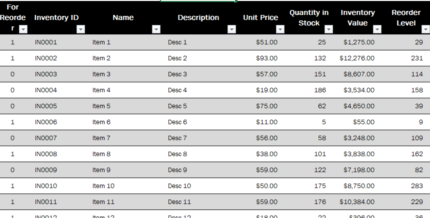
Looking at large amounts of data can be quite straining on the eyes. Thankfully Excel has a useful function to make it easier alternate row styling. Simply put Zebra striping. Although shading rows in alternate colors are a great way to make large amounts of data easier to work with. Well, in this article we are going to tell you how you can shade every other row in Microsoft Excel.
Staring at text and numerals in columns and also a row is not exactly easy on the eyes. There are numerous pre-formed color schemes that you can try. OR you could also just save the hassle of looking through them and elect to color shade alternating lines.
However, don’t worry, you won’t have to color your rows manually. You can apply it all in just a few clicks. Here is how to shade every other row in your file.
First, select your entire table. Then click on Format as Table in the Home tab of your Excel menu.

You will see a series of options and color choices. Pick whichever one you prefer. The presets include options featuring different shades of color, outlines, and head tones. When you have found an option you like. You gotta click on it. The styling will be applied to your table immediately. That’s how you can shade every other row.

Tip: If you want to change the coloring. Then simply repeat the steps and click on a different pre-set as you like.
Conclusion
I hope you guys like this tutorial. I think now you can properly understand how to shade every Other Row in Microsoft Excel and know how to do it. However, if you guys still have some queries and issues related to this article. Then you can ask us in the comments section below. We will get to you shortly. Have a Great Day!


